Show packages used in this analysis
library(tidyverse)
library(here)
library(sf)
library(terra)
library(tmap)
library(patchwork)library(tidyverse)
library(here)
library(sf)
library(terra)
library(tmap)
library(patchwork)With an ever growing human population, marine aquaculture has the potential to play a significant role global food supply, and is a more sustainable option than land-based meat production (Hall et al., 2011). A study that mapped the global potential for marine aquaculture based on multiple constraints (e.g., ship traffic, dissolved oxygen, bottom depth) found that global seafood demand could be met using less than 0.015% of the global ocean area (Gentry et al., 2017).
This analysis aims to determine which Exclusive Economic Zones (EEZ) on the West Coast of the US are best suited to develop marine aquaculture for several species of oysters and Pacific littleneck clams (Leukoma staminea),two of the most common species farmed in marine aquaculture on the West Coast. Suitable growing locations were determined based on range of suitable sea surface temperature (SST) and depth values for each species listed below. Oyster conditions were provided in the assignment description, and suitable temperatures and depths for the littleneck clam were selected based on Shaw (1986) and Harbo (1997). Suitable growing areas for oysters were found first, and then the workflow was made generalizable by transforming into a function that could be used to find suitable growing areas for any marine aquaculture species on the West Coast based on ocean depth and SST.
Suitable growing conditions for oysters:
sea surface temperature: 11-30°Cdepth: 0-70 meters below sea levelSuitable growing conditions for the Pacific littleneck clam:
sea surface temperature: 0-25°Cdepth: 0-46 meters below sea levelAnnual sea surface temperature (SST) from the years 2008 to 2012 were used to characterize the average SST within the region. This data was originally generated from NOAA’s 5km Daily Global Satellite Sea Surface Temperature Anomaly v3.1.
Data files:
average_annual_sst_2008.tifaverage_annual_sst_2009.tifaverage_annual_sst_2010.tifaverage_annual_sst_2011.tifaverage_annual_sst_2012.tifBathymetric data was sourced from General Bathymetric Chart of the Oceans (GEBCO) to characterize the depth of the ocean (m below sea level).
Data file: depth.tif
Maritime boundaries were designated using Exclusive Economic Zones (EEZs) off of the west coast of US from Marine Regions.
Data file: wc_regions_clean.shp
Boundaries for all U.S. states and territories, included for context in the maps, were sourced from NOAA’s national GIS program.
Data file: s_05mr24.shp
Pseudo code/outline:
Prepare data. Load all necessary data, combine the SST data into a raster stack, and make sure they’re all in the same CRS. If not, transform everything to WGS 84 (EPSG:4326).
Process data. Find the mean SST from 2008-2012, convert it from Kelvin to Celsius, resample the bathymetry raster to match the resolution, extent, and position of the SST raster, and crop the depth raster to match the extent of the SST raster.
Find suitable locations. Determine which locations meet the suitable growing conditions for oysters only before expanding the workflow to other species. To do this, we first need to reclassify the bathymetry and SST rasters to either NA (unsuitable), or 1 (suitable). These rasters were then multiplied by each other to isolate areas that meet suitable conditions for both depth and SST.
Determine the most suitable EEZ. Calculate the amount of suitable area for each EEZ region to rank zones by priority. To do this, rasterize the EEZ shapefile, mask it to the suitable locations, calculate the area of each cell in the raster, and sum the area of suitable locations in each EEZ. Lastly, join the area data back to the EEZ shapefile and make some visualizations.
Create a reproducible workflow for other species. After finding locations with suitable growing conditions for oysters, this workflow was transformed into a function that could isolate suitable growing conditions for any marine aquaculture species on the West Coast based on ocean depth and SST. The function has the following characteristics:
We want to load the SST data as a raster stack to make it easier to generate a mean SST raster for the years 2008-2012.
# shapefile for West Coast EEZ
wc_eez <- st_read(here("posts/2024-11-20-aquaculture/data/wc_regions_clean.shp"))

# bathymetry raster
bathy <- rast(here("posts/2024-11-20-aquaculture/data/depth.tif"))

# SST rasters
sst_2008 <- rast(here("posts/2024-11-20-aquaculture/data/average_annual_sst_2008.tif"))
sst_2009 <- rast(here("posts/2024-11-20-aquaculture/data/average_annual_sst_2009.tif"))
sst_2010 <- rast(here("posts/2024-11-20-aquaculture/data/average_annual_sst_2010.tif"))
sst_2011 <- rast(here("posts/2024-11-20-aquaculture/data/average_annual_sst_2011.tif"))
sst_2012 <- rast(here("posts/2024-11-20-aquaculture/data/average_annual_sst_2012.tif"))

# SST raster stack
sst_stack <- c(sst_2008, sst_2009, sst_2010, sst_2011, sst_2012)
#plot(sst_stack)WGS 84 if they don’t match# # check if each dataset has the same CRS
# crs(wc_eez) == crs(bathy)
# crs(wc_eez) == crs(sst_stack)
# crs(bathy) == crs(sst_stack)
# none are in the same CRS; transform all to WGS 84
bathy <- project(bathy,
"EPSG:4326")
sst_stack <- project(sst_stack,
"EPSG:4326")
wc_eez <- st_transform(wc_eez,
crs = st_crs(bathy))
# check if they are now in the same CRS
if(crs(wc_eez) == crs(bathy) & crs(wc_eez) == crs(sst_stack)) {
print("Carry on! All datasets are now in the same CRS")
} else {
warning("STOP! Datasets are not in the same CRS")
}[1] "Carry on! All datasets are now in the same CRS"To prepare the data for the growing suitability analysis, we found the mean SST from 2008-2012, converted it from Kelvin to Celsius, resampled the bathymetry raster to match the resolution, extent, and position of the SST raster using the nearest neighbor method, and cropped the depth raster to match the extent of the SST raster.
# find the mean SST from 2008-2012
# create a single raster of average SST
sst_mean <- mean(sst_stack)
# plot(sst_mean) # QC to make sure this created one raster


# convert average SST from Kelvin to Celsius
# subtract 273.15 from each grid cell in the raster
sst_mean_celsius <- sst_mean - 273.15
# plot(sst_mean_celsius) # QC to make sure this worked


# resample the bathy raster
# match the resolution, extent, and position of the SST raster
bathy_resample <- resample(bathy,
                           sst_mean_celsius,
                           method = "near")


# crop & mask the depth raster to match the extent of the SST raster
bathy_crop <- crop(bathy_resample,
                   sst_mean_celsius,
mask = TRUE)# resolution
if(all(res(bathy_crop) == res(sst_mean_celsius))) {
print("The bathy and SST data have the same resolution.")
} else {
warning("STOP! Resolution does not match.")
}[1] "The bathy and SST data have the same resolution."# extent
if(ext(bathy_crop) == ext(sst_mean_celsius)) {
print("The bathy and SST data have the same extent.")
} else {
warning("STOP! The bathy and SST raster do not have the same extent.")
}[1] "The bathy and SST data have the same extent."# CRS
if(crs(bathy_crop) == crs(sst_mean_celsius)) {
print("The bathy and SST data have the same CRS.")
} else {
warning("STOP! The bathy and SST data do not have the same CRS.")
}[1] "The bathy and SST data have the same CRS."# load US states for context
us_states <- st_read(here("posts/2024-11-20-aquaculture/data/us_states/s_05mr24.shp"),
quiet = TRUE) %>%
filter(STATE %in% c("WA", "CA", "OR", "NV", "ID"))
us_states <- st_make_valid(us_states) %>%
st_transform(crs = st_crs(wc_eez))
bathy_map <- tm_grid(lines = FALSE) +
tm_shape(us_states) +
tm_polygons(col = "grey",
alpha = 0.2,
border.col = "black") +
tm_shape(bathy_crop,
is.main = TRUE) +
tm_raster(palette = "Blues",
breaks = c(-4000, -2000, -1000, -500, -100, -50, 0),
title = "Bathymetry (m)") +
tm_shape(wc_eez) +
tm_borders(col = "black",
lwd = 1.5) +
tm_text("rgn_key", size = 0.7, col = "black") +
tm_layout(legend.outside = TRUE,
frame = TRUE)
bathy_map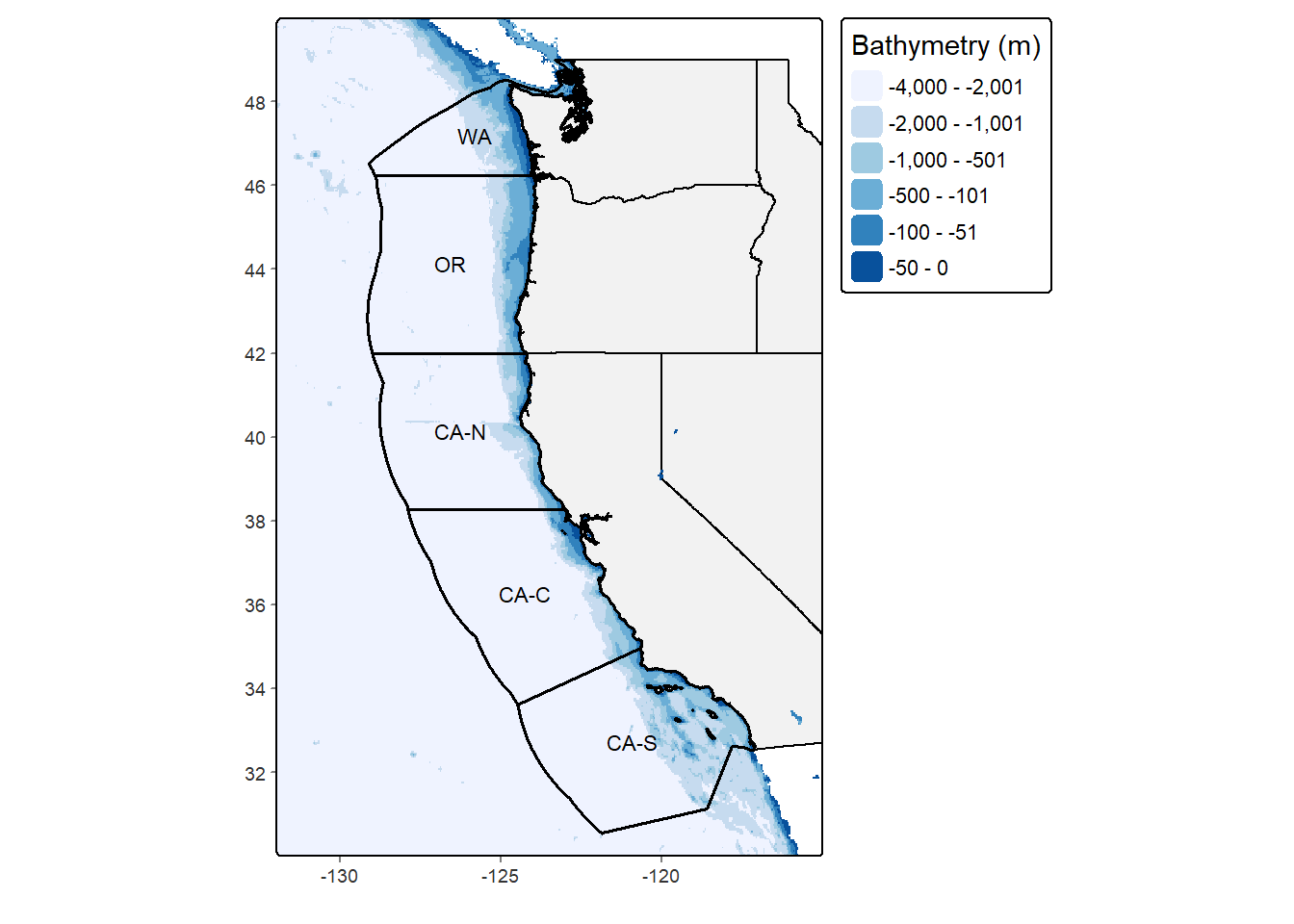
sst_map <- tm_grid(lines = FALSE) +
tm_shape(us_states) +
  tm_polygons(col = "grey",
              alpha = 0.2,
              border.col = "black") +
tm_shape(sst_mean_celsius,
         is.main = TRUE) +
  tm_raster(palette = "viridis",
            style = "cont",
            title = "Sea Surface Temperature (°C)") +
tm_shape(wc_eez) +
  tm_borders(col = "black",
              lwd = 1.5) +
  tm_text("rgn_key", size = 0.7, col = "white") +
  tm_layout(legend.outside = TRUE,
            frame = TRUE)
sst_map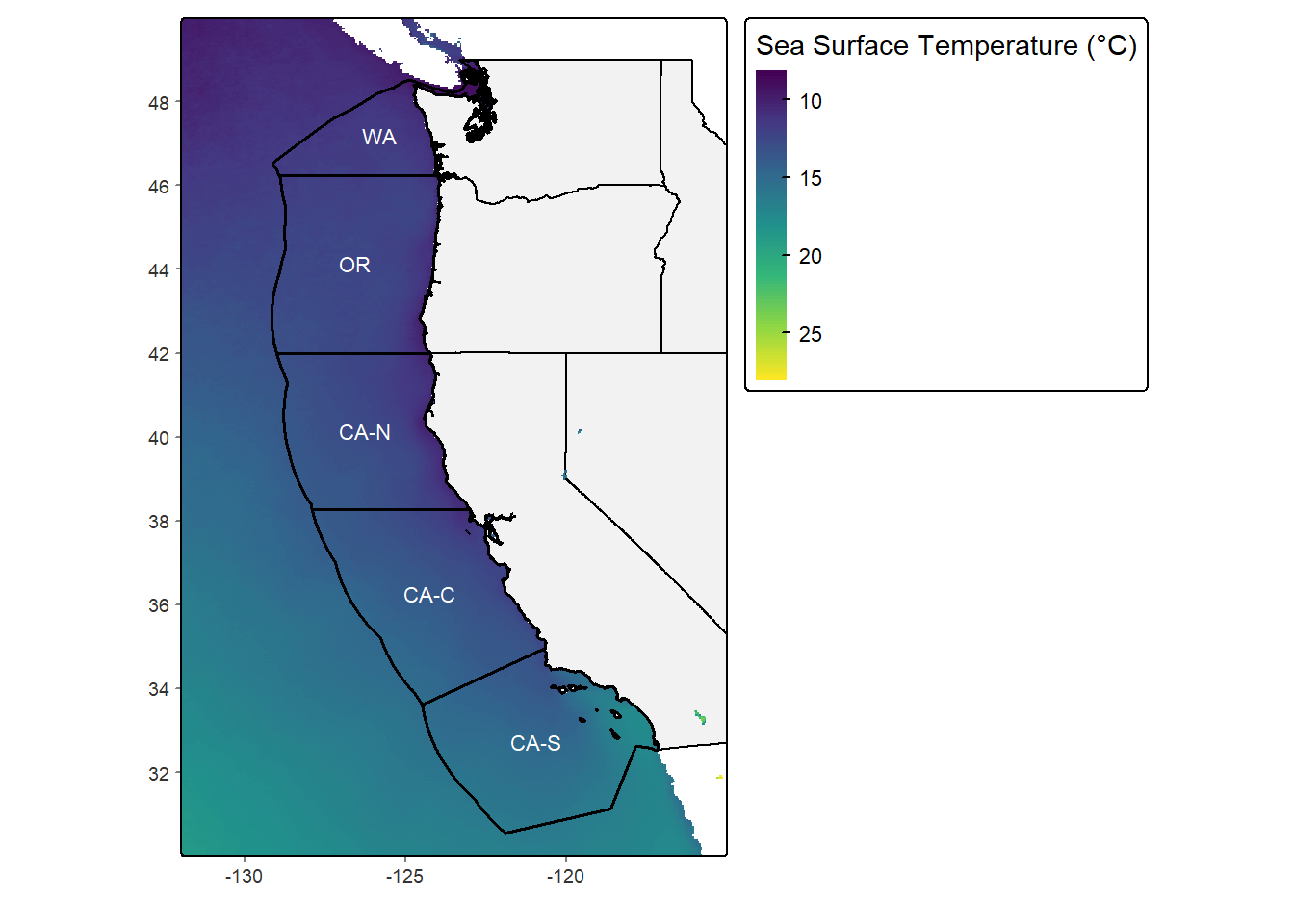
Suitable growing conditions for oysters are defined as follows:
sea surface temperature: 11-30°Cdepth: 0-70 meters below sea levelTo find suitable locations for oysters, we reclassified the SST and depth data into locations that meet the suitable growing conditions for oysters. Suitable areas we defined as 1, and unsuitable areas were assigned NA values. We then used map algebra to multiply the reclassified rasters together to find locations that meet the suitable growing conditions for both depth and SST. If either of these environmental variables’ suitable conditions were not met, the location was assigned a value of NA and considered unsuitable.
# define SST reclassification matrix
rcl_sst <- matrix(c(-Inf, 11, NA,
                    11, 30, 1,
                    30, Inf, NA),
                  ncol = 3,
                  byrow = TRUE)
# define depth reclassification matrix
rcl_depth <- matrix(c(-Inf, -70, NA,
                      -70, 0, 1,
                      0, Inf, NA),
                    ncol = 3,
                    byrow = TRUE)

# reclassify SST and depth data into locations that are suitable for oysters
sst_reclass <- classify(sst_mean_celsius,
                        rcl_sst)
bathy_reclass <- classify(bathy_crop,
                          rcl_depth)


# find locations that meet the suitable growing conditions for oysters
# values of 1 indicate suitable locations for both depth and SST!
oyster_suitable <-  sst_reclass * bathy_reclass
# plot(oyster_suitable)To determine the most suitable EEZ for oysters, we calculated the total area of suitable growing locations in each EEZ region. We first rasterized the EEZ shapefile to mask it to the suitable locations for oysters. Then, we calculated the area of each cell in the raster using the terra::cellSize() function and summed the area of suitable locations in each EEZ with terra::zonal(). Lastly, we joined the area data back to the EEZ shapefile by rgn and calculated the percent of each EEZs total area that has suitable growing areas for oysters.
# rasterize the EEZ shapefile
wc_eez_rast <- rasterize(wc_eez,
                         oyster_suitable,
                         field = "rgn")
# plot(wc_eez_rast) # QC

# crop & mask it to the suitable locations for oysters
wc_eez_suitable <- crop(wc_eez_rast,
                        oyster_suitable,
                        mask = TRUE)

# find the area covered by each cell in the masked EEZ raster
cell_area <- cellSize(wc_eez_suitable,
                      unit = "km")

# calculate the area of suitable locations for oysters in each EEZ
suitable_area <- zonal(cell_area,
                       wc_eez_suitable, # define the zones to calc area in
                       fun = "sum",
                       na.rm = TRUE)

# join the area data back to the EEZ shapefile
wc_eez_joined <- left_join(wc_eez, suitable_area,
                           by = "rgn") %>%
  rename(suitable_area_km2 = area) %>%
  select(rgn, rgn_key, area_km2, suitable_area_km2) %>%
mutate(percent_suitable = suitable_area_km2 / area_km2 * 100)To visualize the results, we made two figures: (1) a map of EEZ regions colored by the amount of suitable area (km^2) for oysters; (2) two bar plots to show the total suitable area (km^2) and the percent of each EEZs total area that has suitable growing areas for oysters.
tm_grid(lines = FALSE) +
tm_shape(us_states) +
  tm_polygons(col = "grey",
              alpha = 0.2,
              border.col = "black") +
tm_shape(wc_eez_joined,
         is.main = TRUE) +
  tm_polygons(col = "suitable_area_km2",
              palette = "Greens",
              title = "Amount of suitable area (km²)",
              style = "cat") +
  tm_text("rgn_key", size = 0.7, col = "black", show.legend = FALSE) +
tm_layout(legend.outside = TRUE,
            frame = TRUE,
            main.title = "Suitable growing area for oysters in West Coast EEZs",
            main.title.size = 1.3)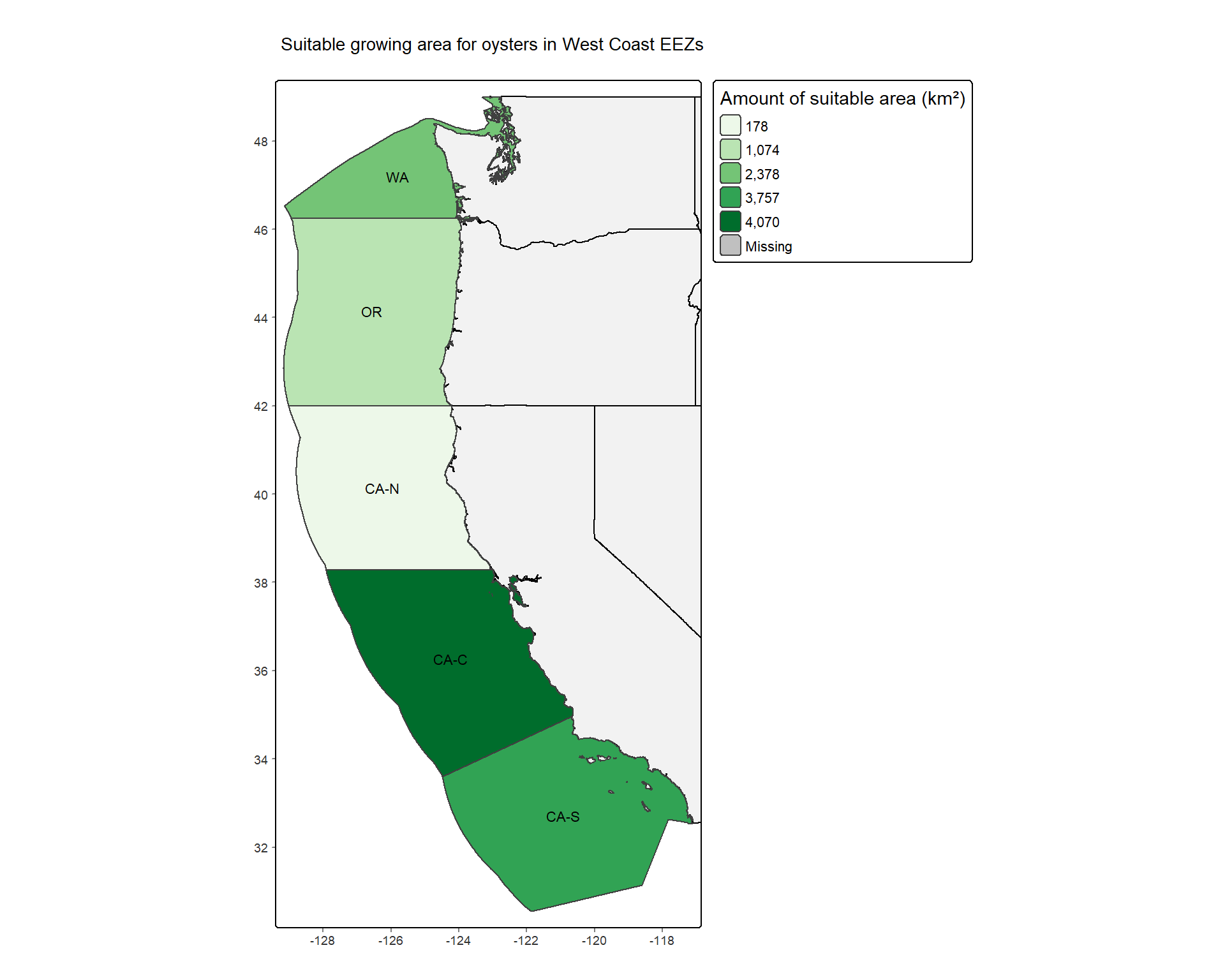
plot1 <- ggplot(wc_eez_joined,
                aes(x = rgn_key,
                    y = suitable_area_km2)) +
  geom_bar(stat = "identity",
           fill = "seagreen3",
           col = "black") +
  labs(title = " ",
       x = "EEZ",
       y = "Suitable area (km^2)") +
  theme_minimal() +
  theme(axis.text.x = element_text(angle = 45,
                                   hjust = 1))
#plot1

plot2 <- ggplot(wc_eez_joined,
                aes(x = rgn_key,
                    y = percent_suitable)) +
  geom_bar(stat = "identity",
           fill = "seagreen4",
           col = "black") +
  labs(title = " ",
       x = "EEZ",
       y = "% suitable growing areas") +
  theme_minimal() +
  theme(axis.text.x = element_text(angle = 45,
                                   hjust = 1))
#plot2

combined_plots <- plot1 + plot2
combined_plots <- combined_plots + plot_annotation(tag_levels = "A")
combined_plots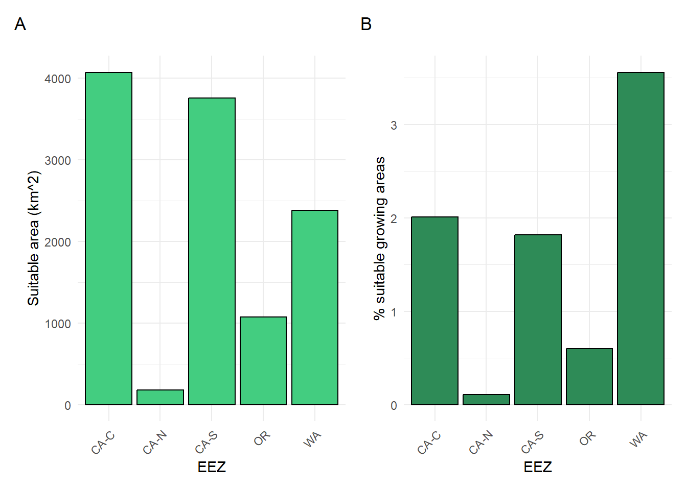
Now that we have a workflow to find suitable growing areas for oysters, we can transform this workflow into a function that can be used to find suitable growing areas for any marine aquaculture species on the West Coast based on ocean depth and SST!
# function to find suitable locations for any marine aquaculture species
ideal_growing_conditions <- function(species, depth_min, depth_max,
                                     sst_min, sst_max){

  ################ reclassification to find suitable habitat ################

  # define SST reclassification matrix
  rcl_sst <- matrix(c(-Inf, sst_min, NA,
                      sst_min, sst_max, 1,
                      sst_max, Inf, NA),
                    ncol = 3,
                    byrow = TRUE)
  # define depth reclassification matrix
  rcl_depth <- matrix(c(-Inf, depth_max, NA,
                        depth_max, depth_min, 1,
                        depth_min, Inf, NA),
                      ncol = 3,
                      byrow = TRUE)


  # reclassify SST data into suitable locations
  sst_reclass <- classify(sst_mean_celsius,
                          rcl_sst)
  # reclassify depth data into suitable locations
  bathy_reclass <- classify(bathy_crop,
                            rcl_depth)


  # find locations that meet the suitable growing conditions
  suitable_locations <-  sst_reclass * bathy_reclass


  ##################### finding the most suitable EEZ #####################

  # rasterize the EEZ shapefile
  wc_eez_rast <- rasterize(wc_eez,
                           suitable_locations,
                           field = "rgn")

  # crop & mask it to the suitable locations
  wc_eez_suitable <- crop(wc_eez_rast,
                          suitable_locations,
                          mask = TRUE)

  # find the area of each cell in the masked EEZ raster
  cell_area <- cellSize(wc_eez_suitable,
                        unit = "km")

  # calculate the area of suitable locations in each EEZ
  suitable_area <- zonal(cell_area,
                         wc_eez_suitable,
                         fun = "sum",
                         na.rm = TRUE)

  # join the area data back to the EEZ shapefile
  wc_eez_joined <- left_join(wc_eez,
                             suitable_area,
                             by = "rgn") %>%
    rename(suitable_area_km2 = area) %>%
    select(rgn, rgn_key, area_km2, suitable_area_km2) %>%
    mutate(percent_suitable = suitable_area_km2 / area_km2 * 100)


  ##################### mapping the results #####################

  # map of EEZ regions colored by the amount of suitable area

  tm_grid(lines = FALSE) +
  tm_shape(us_states) +
  tm_polygons(col = "grey",
              alpha = 0.2,
              border.col = "black") +
  tm_shape(wc_eez_joined,
           is.main = TRUE) +
    tm_polygons(col = "suitable_area_km2",
                palette = "Greens",
                title = "Amount of suitable area (km²)",
                style = "cat") +
    tm_text("rgn_key", size = 0.7, col = "black", show.legend = FALSE) +
    tm_layout(legend.outside = TRUE,
              frame = TRUE,
              main.title = paste("Suitable growing area for", species,
                            "in West Coast EEZs"),
              main.title.size = 2)

}# test the function with the Pacific littleneck clam's growing conditions
ideal_growing_conditions(species = "Pacific littleneck clams",
depth_min = 0,
depth_max = -46,
sst_min = 0,
sst_max = 25)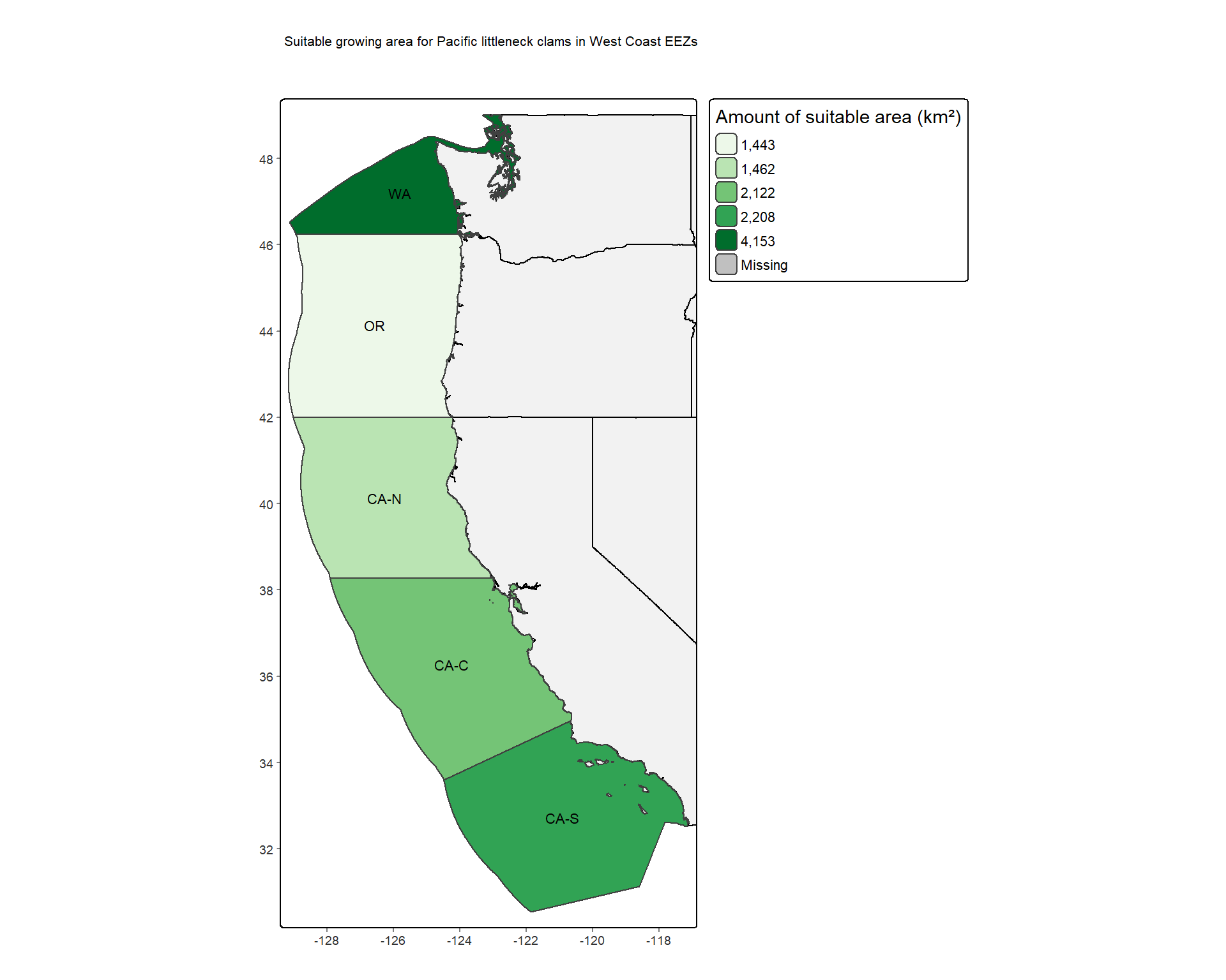
Looking at Figure 4, we can see that the central California EEZ (CA-C) has the greatest area of suitable growing locations for oysters based on SST and depth, and the Washington EEZ has the greatest percentage of suitable growing locations compared to the EEZs total area. Looking at Figure 5, we can see that the Washington EEZ has both the greatest area of suitable growing locations and the greatest percentage of suitable growing locations for the Pacific littleneck clam.
As the human population continues to grow, the demand for seafood is expected to increase. Marine aquaculture has the potential to play a significant role in meeting this demand, and is a more sustainable option than land-based meat production. This analysis aimed to determine which Exclusive Economic Zones (EEZ) on the West Coast of the US are best suited to develop marine aquaculture for several species of oysters and the Pacific littleneck clam. We only considered two species and two variables driving suitable growing conditions in this analysis, but the workflow can be easily adapted to other species and additional predictor variables to create more robust suitability modeling.
This assignment was created and organized Ruth Oliver, an Assistant Professor at the Bren School and the instructor for EDS 223. EDS 223 (Geospatial Analysis & Remote Sensing) is offered in the Master of Environmental Data Science (MEDS) program at the Bren School.
Flanders Marine Institute (2023). Maritime Boundaries Geodatabase: Maritime Boundaries and Exclusive Economic Zones (200NM), version 12. Available online at https://www.marineregions.org/. https://doi.org/10.14284/632
GEBCO Compilation Group (2024) GEBCO 2024 Grid (doi:10.5285/1c44ce99-0a0d-5f4f-e063-7086abc0ea0f)
Gentry, R. R., Froehlich, H. E., Grimm, D., Kareiva, P., Parke, M., Rust, M., Gaines, S. D., & Halpern, B. S. Mapping the global potential for marine aquaculture. Nature Ecology & Evolution, 1, 1317-1324 (2017).
Hall, S. J., Delaporte, A., Phillips, M. J., Beveridge, M. & O’Keefe, M. Blue Frontiers: Managing the Environmental Costs of Aquaculture (The WorldFish Center, Penang, Malaysia, 2011).
Harbo, R. M. (1997). Shells & shellfish of the Pacific northwest: a field guide. Madiera Park, BC: Harbour Publishing.
NOAA Coral Reef Watch. 2019, updated daily. NOAA Coral Reef Watch Version 3.1 Daily 5km Satellite Regional Virtual Station Time Series Data for Southeast Florida, Mar. 12, 2013-Mar. 11, 2014. College Park, Maryland, USA: NOAA Coral Reef Watch. Data set accessed at https://coralreefwatch.noaa.gov/product/vs/data.php.
Shaw, W N. (1986) Species profiles: life histories and environmental requirements of coastal fishes and invertebrates (Pacific Southwest): Common littleneck clam. Protothaca staminea. United States.
@online{pepperdine2024,
  author = {Pepperdine, Maxwell},
  title = {Assessing Marine Aquaculture Suitability on the {West}
    {Coast}},
  date = {2024-11-18},
  url = {https://maxpepperdine.github.io/posts/2024-11-20-aquaculture/},
  langid = {en}
}