Code
library(tidyverse)
library(here)
library(nlraa)
library(janitor)
library(tibble)
library(kableExtra)
library(knitr)
library(Metrics)
library(nls2)
library(broom)
library(tidyverse)
library(here)
library(nlraa)
library(janitor)
library(tibble)
library(kableExtra)
library(knitr)
library(Metrics)
library(nls2)
library(broom)Data Description:
The data used in this analysis comes from the paper “Nonlinear Regression Models and Applications in Agricultural Research,” written by Sotirios Archontoulis and Fernando Miguez. It’s stored in an object called sm in the nlraa package, and contains the following 5 variables:
variable <- c("doy", "block", "input", "crop", "yield")
data_type <- c("integer", "integer", "integer", "factor", "numeric")
description <- c("day of the year, spanning 141-303",
                 "1-4 blocks used in the experiment",
                 "low (1) or high (2) agronomic input",
                 "three levels: fiber sorghum (F), sweet sorghum (S), and maize (M)",
                 "biomass yield in Mg/ha")

sm_variables <- tibble(Variable = variable,
                           Data.Type = data_type,
                           Description = description)

kable(sm_variables, col.names = c("Variable", "Data Type",
                                  "Description")) %>%
kable_classic_2() sm object from the nlraa package.
| Variable | Data Type | Description |
|---|---|---|
| doy | integer | day of the year, spanning 141-303 |
| block | integer | 1-4 blocks used in the experiment |
| input | integer | low (1) or high (2) agronomic input |
| crop | factor | three levels: fiber sorghum (F), sweet sorghum (S), and maize (M) |
| yield | numeric | biomass yield in Mg/ha |
Objective:
To maximize yield, it’s crucial for farmers to understand the biology of plants and their responses to fertilizers. This analysis aims to help farmers make predictions on their yields by running non-linear least squares on experimental growth data for three grains in Greece.
Data Citation:
Archontoulis, S.V. and Miguez, F.E. (2015), Nonlinear Regression Models and Applications in Agricultural Research. Agronomy Journal, 107: 786-798. https://doi.org/10.2134/agronj2012.0506
Psuedo-code:
sm from the nlraa package.purrrsm_raw <- nlraa::sm
sm_df <- sm_raw %>%
clean_names()\[ Y=Y_{max}(1 + \frac{t_e-t}{t_e-t_m})(\frac{t}{t_e})^\frac{t_e}{t_e-t_m} \]
beta <- function(ymax,doy,tm,te){
  out=ymax*(1 + ((te-doy)/(te-tm)))*((doy/te)^(te/(te-tm)))
return(out)
}guess_plot <- ggplot(sm_df, aes(x = doy, y = yield,
shape = crop, color = crop)) +
geom_point() +
facet_wrap(~input) +
theme_bw()
#guess_plotymax_guess = max(sm_df$yield)
tm_guess = 225
te_guess = 260sorghum_df <- sm_df %>%
filter(input == 2 & crop == "S")sorghum_nls=nls(formula=yield~beta(ymax,doy,tm,te),
data=sorghum_df,
start=list(ymax=ymax_guess, tm=tm_guess,
te=te_guess),
trace=TRUE)
# sorghum_nlstidy(sorghum_nls) %>%
kable(col.names = c("Parameter", "Selected Value",
"Standard Error", "Statistic", "p-value")) %>%
kable_classic_2()| Parameter | Selected Value | Standard Error | Statistic | p-value |
|---|---|---|---|---|
| ymax | 39.82035 | 2.248860 | 17.70690 | 0 |
| tm | 244.77725 | 3.511964 | 69.69811 | 0 |
| te | 281.58631 | 2.080764 | 135.32834 | 0 |
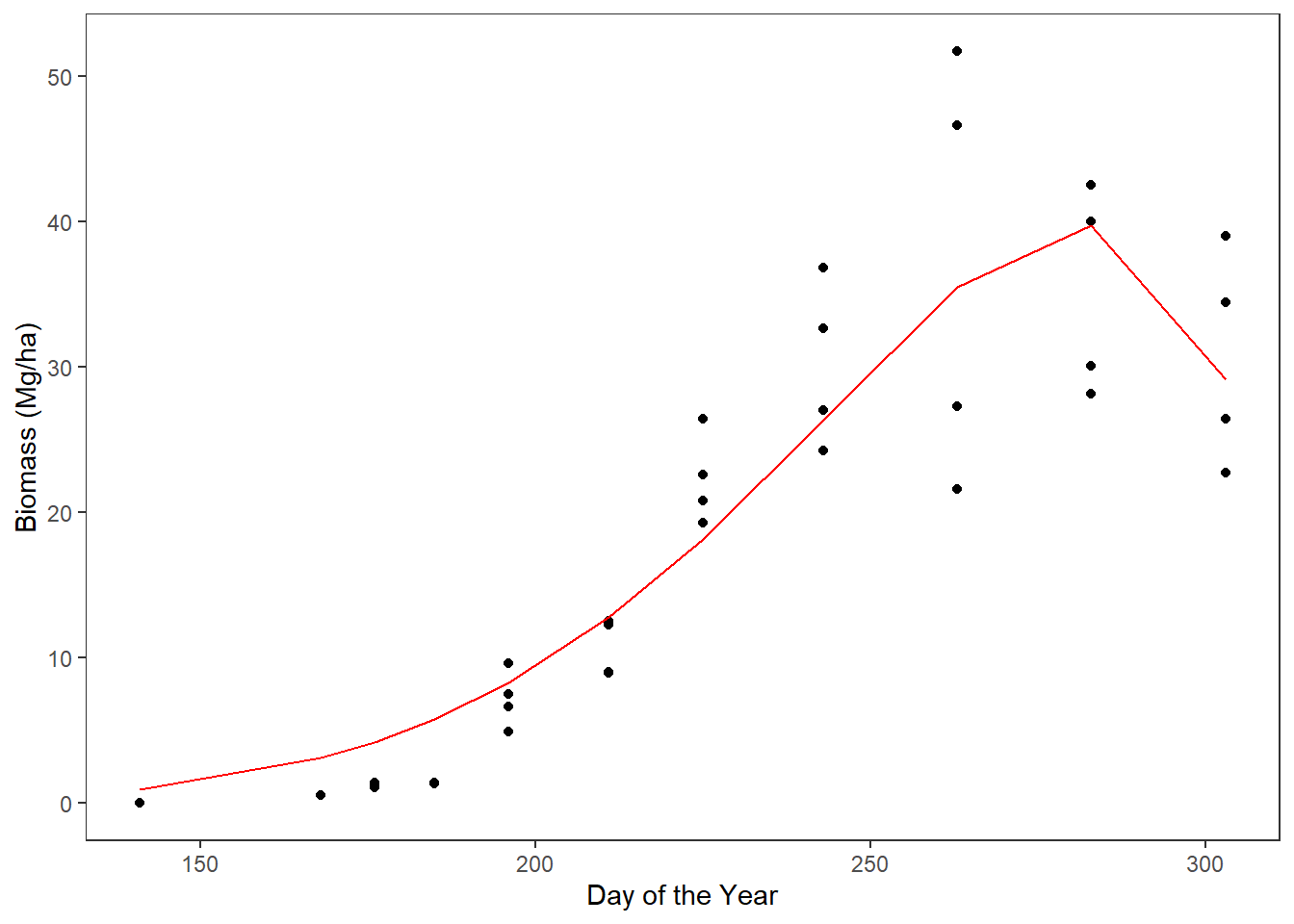
# find the sorghum_nls model predictions
sorghum_predict <- sorghum_df %>%
  mutate(predict = predict(sorghum_nls, newdata = sorghum_df))

# plot the sorghum_nls model on top of the sweet sorghum data
ggplot(data = sorghum_predict) +
  geom_point(aes(x = doy, y = yield)) +
  geom_path(aes(x = doy, y = predict), color = 'red') +
  theme_bw() +
  labs(x = "Day of the Year",
       y = "Biomass (Mg/ha)") +
  theme(
    panel.grid.major = element_blank(),
    panel.grid.minor = element_blank()
  )
#Define a new function to pass along all nls calls

all_nls_fcn<-function(sm_df){

  ymax_guess=max(sm_df$yield)
  tm_guess=225
  te_guess=260

  nls(yield~beta(ymax,doy,tm,te),
    data=sm_df,
    start=list(ymax=ymax_guess, tm=tm_guess,
                             te=te_guess))
}# run nls models for all 24 combinations of plot, input level, crop type
# calculate RMSE values
beta_all <- sm_df %>%
group_by(input, crop, block) %>%
nest() %>%
mutate(nls_model = map(data, ~all_nls_fcn(.x))) %>%
mutate(predictions = map2(nls_model, data,
~predict(.x, newdata = .y))) %>%
mutate(RMSE = map2_dbl(predictions, data,
~Metrics::rmse(.x, .y$yield))) %>%
mutate(smooth = map(nls_model,
~predict(.x, newdata = list(doy = seq(147, 306)))))
#'smooth' breakdown:
### runs the model between every single 'doy' point
### creates a smoothed line of the best fitting NLS model ### Fiber Sorghum (F) ###
beta_fiber <- beta_all %>%
filter(crop == "F")
best_fiber = min(beta_fiber$RMSE)
#pull out the model to make tables
best_fiber1 <- beta_all$nls_model[22]
### Sweet Sorghum (S) ###
beta_sweet <- beta_all %>%
filter(crop == "S")
best_sweet = min(beta_sweet$RMSE)
#pull out the model to make tables
best_sweet1 <- beta_all$nls_model[14]
### Maize (M) ###
beta_maize <- beta_all %>%
filter(crop == "M")
best_maize = min(beta_maize$RMSE)
#pull out the model to make tables
best_maize1 <- beta_all$nls_model[4]# add RMSE values into the table caption
### Fiber ###
tidy(best_fiber1[[1]]) %>%
kable(col.names = c("Variable", "Parameter Values",
"Standard Error", "Statistic",
"p-value")) %>%
kable_classic_2()
### Sweet ###
tidy(best_sweet1[[1]]) %>%
kable(col.names = c("Variable", "Parameter Values",
"Standard Error", "Statistic",
"p-value")) %>%
kable_classic_2()
### Maize ###
tidy(best_maize1[[1]]) %>%
kable(col.names = c("Variable", "Parameter Values",
"Standard Error", "Statistic",
"p-value")) %>%
kable_classic_2()| Variable | Parameter Values | Standard Error | Statistic | p-value |
|---|---|---|---|---|
| ymax | 29.05639 | 1.657636 | 17.52881 | 5e-07 |
| tm | 244.99880 | 3.538539 | 69.23727 | 0e+00 |
| te | 280.42964 | 1.838951 | 152.49433 | 0e+00 |
| Variable | Parameter Values | Standard Error | Statistic | p-value |
|---|---|---|---|---|
| ymax | 31.34741 | 2.047998 | 15.30637 | 1.2e-06 |
| tm | 245.77425 | 3.815015 | 64.42288 | 0.0e+00 |
| te | 278.34654 | 1.817123 | 153.17984 | 0.0e+00 |
| Variable | Parameter Values | Standard Error | Statistic | p-value |
|---|---|---|---|---|
| ymax | 18.93109 | 0.8396967 | 22.54516 | 5e-07 |
| tm | 225.22836 | 1.9262857 | 116.92365 | 0e+00 |
| te | 252.57495 | 1.8691829 | 135.12586 | 0e+00 |
# filtered the data and unnest the smoothed values for plotting
# add a doy column
unnest_df <- beta_all %>%
  filter(block == 1) %>%
  tidyr::unnest(smooth) %>%
  mutate(doy = seq(147, 306)) %>%
  filter(!(doy > 263 & crop == "M"))

# filter the original data for plotting on top of model results
sm_filter <- sm_df %>%
  filter(block == 1) %>%
  select(doy, yield, crop)

# # join the unnest_df to the sm_filter to get yield data for fun
# unnest_sm_join <- left_join(unnest_df, sm_filter,
#                             by = join_by(doy))

# # unnest the model predictions
# predict_df <- beta_all %>%
# tidyr::unnest(predictions)# change the facet labels from "1" and "2" to "low" and "high"
unnest_df$input <- factor(unnest_df$input, levels = c(1, 2),
labels = c("Low", "High"))
# make the final plot
final_plot <- ggplot() +
geom_path(data = unnest_df, aes(x = doy, y = smooth, color = crop)) +
geom_point(data = sm_filter, aes(x = doy, y = yield, shape = crop),
size = 1.5, color = "darkslategrey") +
facet_wrap(~input) +
theme_bw() +
labs(x = "Day of the Year",
y = "Biomass (Mg/ha)",
color = "Model Fit",
shape = "sm Data") +
theme(
panel.grid.major = element_blank(),
panel.grid.minor = element_blank()
)
final_plot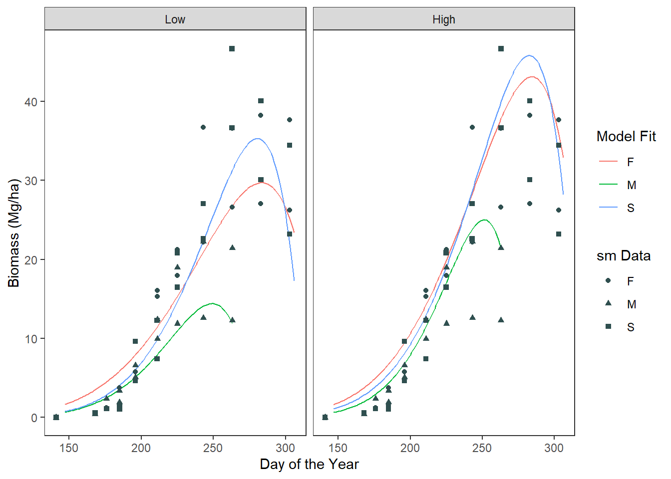
This assignment was created and organized by Nathan Grimes at the Bren School for ESM 244 (Advanced Data Analysis for Environmental Science & Management). ESM 244 is offered in the Master of Environmental Science & Management (MESM) program.
@online{pepperdine2024,
  author = {Pepperdine, Maxwell},
  title = {Maximizing Crop Yields with Data Analysis},
  date = {2024-02-15},
  url = {https://maxpepperdine.github.io/posts/2024-02-15-nonlinear-squares/},
  langid = {en}
}