Comparing water chemistry in Santa Barbara streams with a cluster analysis

SBC LTER Logo. Image credit: SBC LTER

Overview

Data Description:

The data used in this analysis is a data package from Santa Barbara Coastal (SBC) Long Term Ecological Research (LTER). It contains stream water chemistry measurements taken in various watersheds throughout the Santa Barbara area, with data collection beginning in 2000. As described by the data source, this “dataset is ongoing, and data will be added approximately annually. Stream water samples are collected weekly during non-storm flows in winter, and bi-weekly during summer. During winter storms, samples are collected hourly (rising limb) or at 2-4 hour intervals (falling limb). Analytes sampled in the SBC LTER watersheds include dissolved nitrogen (nitrate, ammonium, total dissolved nitrogen); soluble reactive phosphorus (SRP); particulate organic carbon, nitrogen and phosphorus; total suspended sediments; and conductivity.”

Data Citation:

Santa Barbara Coastal LTER and J. Melack. 2019. SBC LTER: Land: Stream chemistry in the Santa Barbara Coastal drainage area, ongoing since 2000 ver 16. Environmental Data Initiative. https://doi.org/10.6073/pasta/67a558a24ceed9a0a5bf5e46ab841174

Objective:

This analysis aims to use complete linkage agglomerative hierarchical clustering to compare water chemistry by specific sites in the SBC LTER dataset. This “bottom-up” approach to clustering will allow us to group sites whose water quality are more similar to each other and different from other sites in the dataset.

Pseudo-code:

• Load the data.
• Examine which columns have a lot of NA’s and drop them from the analysis. Use the summary() function to identify all columns that have greater than 50% NA values and remove them.
• Make a data frame that has a single summary row per site based on the average of all observations from that site. Use na.rm = TRUE when summarizing to remove any rows with NA’s.
• Scale the average measurements at each site.
• Perform the complete linkage agglomerative hierarchical clustering:
  • Calculate the Euclidean distance.
  • Use the stats::hclust() function to perform the complete linkage agglomerative hierarchical clustering.
• Make a clean dendrogram to show the results of the multivariate clustering.

Setup

Load Packages

library(tidyverse)
library(here)
library(janitor)
library(NbClust) #cluster package
library(cluster)
library(dendextend)
library(ggdendro)
library(factoextra)

Load Data

# load the data and assign all values of -999.0 as NA 
stream_chem_raw <- read_csv(here("posts/2024-02-14-hierarchical-cluster/data/sbc_lter_registered_stream_chemistry.csv"), 
                            na = '-999')

Hierarchical Cluster Analysis (by Complete Linkage)

Data Wrangling

Process to Deal w/ NAs:

1. Identify columns with lots of NA values (>50%) using the summary() function, and drop them from the analysis.
2. Use na.rm = TRUE when summarizing water quality measurements at each site to remove all other NA values remaining in the data. I chose this method instead of using drop_na() for the entire data frame because this removed NAs for each respective measurement when calculating their mean values rather than the entire row of data wherever an NA value was present.

# examine which columns have more than 50% NA values 
summary(stream_chem_raw) ## 'tpc_uM' ; 'tpn_uM' ; 'tpp_uM ; 'tss_mgperLiter' 


# drop columns with > 50% NA's from the df
stream_chem_df <- stream_chem_raw %>% 
  select(site_code, nh4_uM, no3_uM, po4_uM, tdn_uM, tdp_uM, spec_cond_uSpercm)


# make a data frame with a single summary row per site 
# take the mean of all observations at each site
# drop NAs using `na.rm = TRUE` when summarizing
### use this df when calculating the Euclidian distance ###
stream_chem_means <- stream_chem_df %>% 
  group_by(site_code) %>% 
  summarize(nh4_avg = mean(nh4_uM, na.rm = TRUE),
            no3_avg = mean(no3_uM, na.rm = TRUE), 
            po4_avg = mean(po4_uM, na.rm = TRUE), 
            tdn_avg = mean(tdn_uM, na.rm = TRUE), 
            tdp_avg = mean(tdp_uM, na.rm = TRUE), 
            spec_avg = mean(spec_cond_uSpercm, na.rm = TRUE))


# scale the average measurements at each site
stream_mean_scale <- stream_chem_means %>% 
  select(-site_code) %>% 
  scale()


### If I want to drop all NA's instread of using na.rm in summarize() ###

# # drop all rows with NA's
# stream_complete <- stream_chem_df %>% 
#   drop_na()
# 
# # scale the measurements at each site
# stream_scale <- stream_complete %>% 
#   scale() # this function centers and/or scales the columns of a numeric matrix
# 
# # compare the scaled and complete df's
# summary(stream_complete)
# summary(stream_scale) # the mean measurement at each site is 0 

Complete Linkage

### complete ###

# calculate Euclidean distance; should this be using the mean stream df???
stream_dist <- dist(stream_mean_scale, method = "euclidean")

# Hierarchical clustering (complete linkage) 
stream_hc_complete <- hclust(stream_dist, method = "complete")

# # Plot it (base plot):
# plot(stream_hc_complete, cex = 0.6, hang = -1)

Make Dendrograms with ggplot

# prep vectors for labelling 
stream_sites <- c("AB00", "AT07", "BC02", "DV01", "GV01", "HO00", "MC00", 
                  "MC06", "ON02", "RG01", "RS02", "SP02", "TO02")

int_placeholders <- c(4, 3, 2, 1, 7, 12, 5, 8, 13, 10, 9, 6, 11)


# make the dendrogram
ggdendrogram(stream_hc_complete) + 
  theme_classic() + 
  scale_x_continuous(labels = stream_sites, breaks = int_placeholders) +
  labs(x = "Measurement site", 
       y = "Distance between clusters")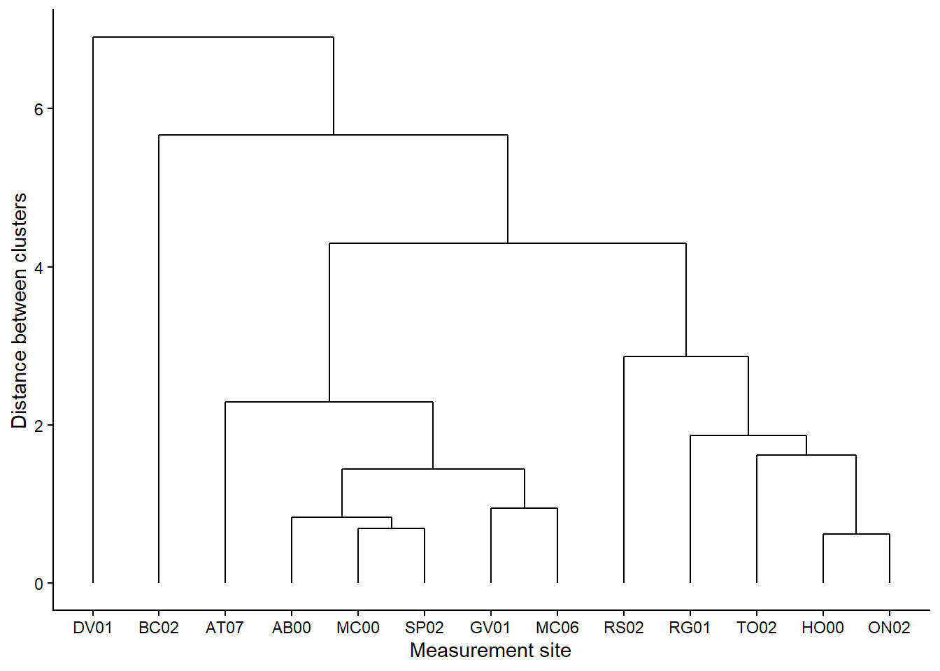

Figure 1: Dendrogram showing the results of the complete linkage agglomerative hierarchical clustering to compare water chemistry by specific sites in the SBC LTER dataset. Each site is shown on the x-axis, and the distance between clusters on the y-axis.

Summary

• For this analysis, we performed complete linkage agglomerative hierarchical clustering to compare water chemistry by specific sites in the SBC LTER dataset. In this method of clustering, all sites start as their own cluster, and are grouped into larger clusters according to similarities between them.
• The height at which branches merge and objects (different sites) exist on the dendrogram indicates the relative dissimilarity between the sites (clusters) being merged. The taller the branch or height at which two clusters merge, the less similar the sites are.
• Looking at the dendrogram in Figure 1 above, we can see that the water chemistry at sites ‘DV01’ and ‘BC02’ are most different from the rest of the sites.
• The smaller groupings of branches and branches closer to eachother might indicate sites in the same watershed or those in a closer spatial proximity with more similar water chemistry measurements.

Acknowledgements

This assignment was created and organized by Casey O’Hara at the Bren School for ESM 244 (Advanced Data Analysis for Environmental Science & Management). ESM 244 is offered in the Master of Environmental Science & Management (MESM) program.