Time series analysis

Overview

Willamette Falls Fish Ladder on the Willamette River (Oregon). Image credit: PGE.

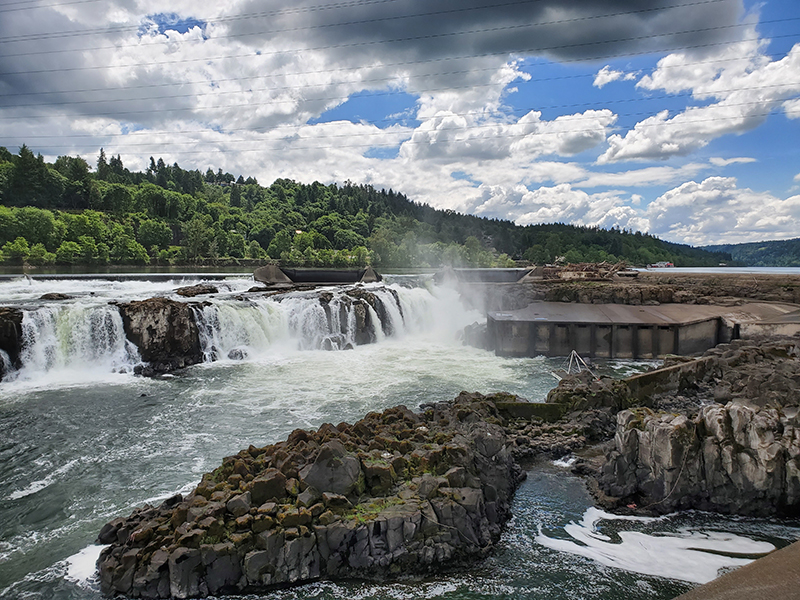
Dataset & report summary: Data used in this analysis was accessed from Columbia River Data Access in Real Time (DART). Columbia River DART provides interactive data resources to support research and management practices relating to the Columbia River Basin salmon populations and overall river ecosystem. This dataset includes information on adult fish passage recorded from 2001-01-01 to 2010-12-31 at the Willamette Falls fish ladder on the Willamette River (Oregon). The following report includes a time series analysis for the data and various figures in three different parts: part 1 (original time series analysis), part 2 (season plots exploring patterns in seasonality), and part 3 (annual counts of fish passage by each species).

Data citation: Columbia Basin Research. (n.d.). Columbia River DART. Retrieved January 25, 2023, from https://www.cbr.washington.edu/dart/query/adult_graph_text

Add Packages and Load Data

library(tidyverse)
library(here)
library(tsibble) #for time series analysis
library(feasts) #feature extraction and statistics for time series
library(fable)
library(patchwork)
library(janitor)

fish_df <- read_csv(here("posts/2024-01-20-salmon-time-series/data/willamette_fish_passage.csv")) %>% 
  clean_names()

Part 1: Original Time Series

#Select the appropriate columns and pivot the data
#Convert the data frame into time series format 
fish_ts <- fish_df %>% 
  select(project, date, coho, jack_coho, steelhead) %>% 
  pivot_longer(cols = 3:5, 
               names_to = "species", values_to = "count") %>% 
  mutate(date = lubridate::mdy(date)) %>% 
  as_tsibble(key = species,
             index = date)

fish_ts_0 <- replace(fish_ts, is.na(fish_ts), 0) #replace NAs with 0

passage_plot <- ggplot(fish_ts_0, 
                       aes(x = date, y = count)) +
  geom_line() +
  theme_bw() +
  facet_wrap(~species, labeller = labeller(species = c(
    "coho" = "Coho", 
    "jack_coho" = "Jack coho", 
    "steelhead" = "Steelhead"))) +
  labs(x = "Year", y = "Fish passage counts") 

  # scale_color_manual(values = c("coho" = "lightblue",
  #                               "jack_coho" = "skyblue2",
  #                               "steelhead" = "skyblue4"))
passage_plot

# passage_plot2 <- ggplot(fish_ts_0, 
#                        aes(x = date, y = count, fill = species)) +
#   geom_col() +
#   theme_bw() +
#   scale_fill_brewer(palette = "Dark2")
# passage_plot2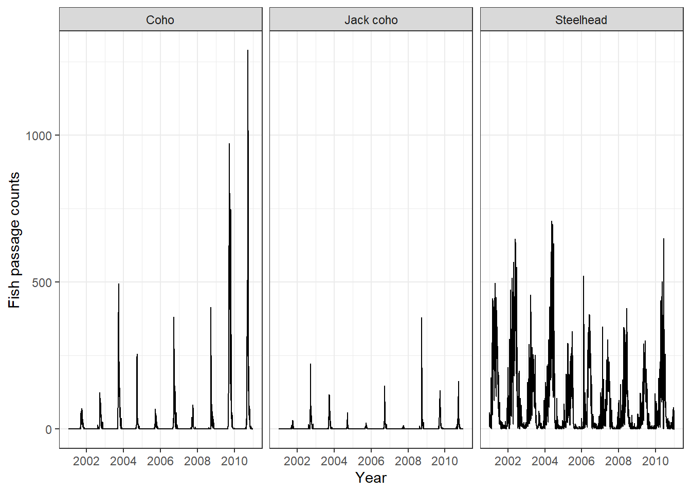

Figure 1: Static plot of adult fish passage for coho, jack coho, and steelhead salmon at the Willamette Falls fish ladder on the Willamette River (Oregon) between 2001-2010.

Major Trends:

• Coho salmon have an increasing trend of fish passage counts, jack coho have a fairly consistent trend, and steelhead have a slightly decreasing trend.
• All three fish species show consistent patterns of seasonality. Coho and jack coho fish passage counts increase significantly in what appears to be later months of each year. This is expected as, according to NOAA, Pacific coho salmon usually return to spawning grounds between September and December. It’s interesting to note that some years have significantly smaller counts during spawning season. The seasonality of increased steelhead counts are more consistent than the coho species, and spread out over a larger spawning season which, according to NOAA, is between the months of April-June.

Part 2: Season Plots

fish_ts_0 %>% 
  gg_season(y = count, pal = hcl.colors(n = 10)) +
  facet_wrap(~species, scales = "free_y", nrow = 3, 
             labeller = labeller(species = c("coho" = "Coho", 
                                             "jack_coho" = "Jack coho", 
                                             "steelhead" = "Steelhead"))) +
  labs(x = "Month", 
       y = "Fish passage counts") +
  theme_bw()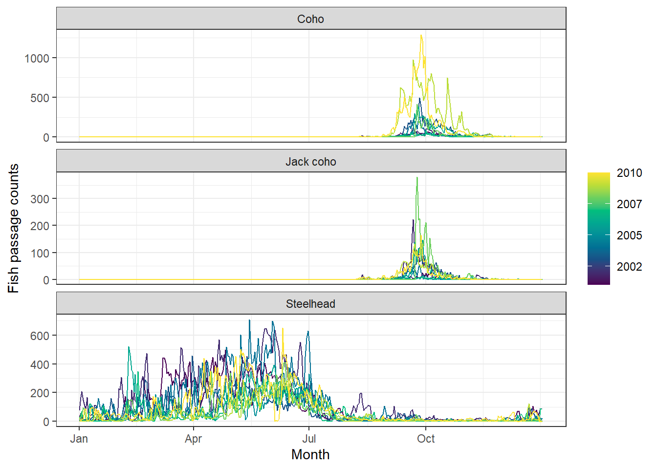

Figure 2: Season plots for coho, jack coho, and steelhead salmon species at the Willamette Falls fish ladder on the Willamette River (Oregon) between 2001-2010. Months are shown on the x-axis and number of fish passage counts on the y-axis, and each year in which data was collected are shown by different colors.

Major Trends:

• The seasonality patterns identified in Figure 1 are much more evident in the season plots above. Fish passage counts for both coho species increase significantly during their spawning season (September-December), which is a much more concentrated time than the steelhead. We also see that coho fish passage counts (shown in the top panel) increased a lot from 2007-2010.
• Seasonality for steelhead fish passage counts is much more spread out than the two coho species, reflective of their longer spawning season (April-June). There is no noticeable trend in changes in fish passage counts between each year data was collected.

Part 3: Annual Counts by Species

fish_ts_annual <- fish_df %>% 
  select(project, date, coho, jack_coho, steelhead) %>% 
  pivot_longer(cols = 3:5, 
               names_to = "species", values_to = "count")

fish_ts_annual_0 <- replace(fish_ts_annual, is.na(fish_ts_annual), 0)

fish_ts_annual_0 <- fish_ts_annual_0 %>% 
  mutate(date = lubridate::mdy(date)) %>% 
  mutate(year = lubridate::year(date)) %>% 
  mutate(Year = as.factor(year)) %>% 
  select(Year, species, count)

fish_count <- aggregate(count ~ Year+species, data = fish_ts_annual_0, FUN = sum)
  
  #group_by(Year, species) %>% 
  #summarize(annual_count = n(), .groups = "drop")

annual_count <- ggplot(fish_count, aes(x = Year, y = count, fill = species)) +
  geom_col(color = "black", size = 0.1) +
  labs(x = "Year", 
       y = "Fish passage counts") +
  theme_bw() +
  facet_wrap(~species, scales = "free_y", nrow = 3, 
             labeller = labeller(species = c("coho" = "Coho", 
                                             "jack_coho" = "Jack coho", 
                                             "steelhead" = "Steelhead"))) +
  scale_fill_brewer() +
  theme(axis.text.x = element_text(angle = 45, hjust = 1)) +
  theme(legend.position = "none") #get rid of the legend
  # geom_text(aes(label = count), vjust = -0.5, size = 2) #show the column values

annual_count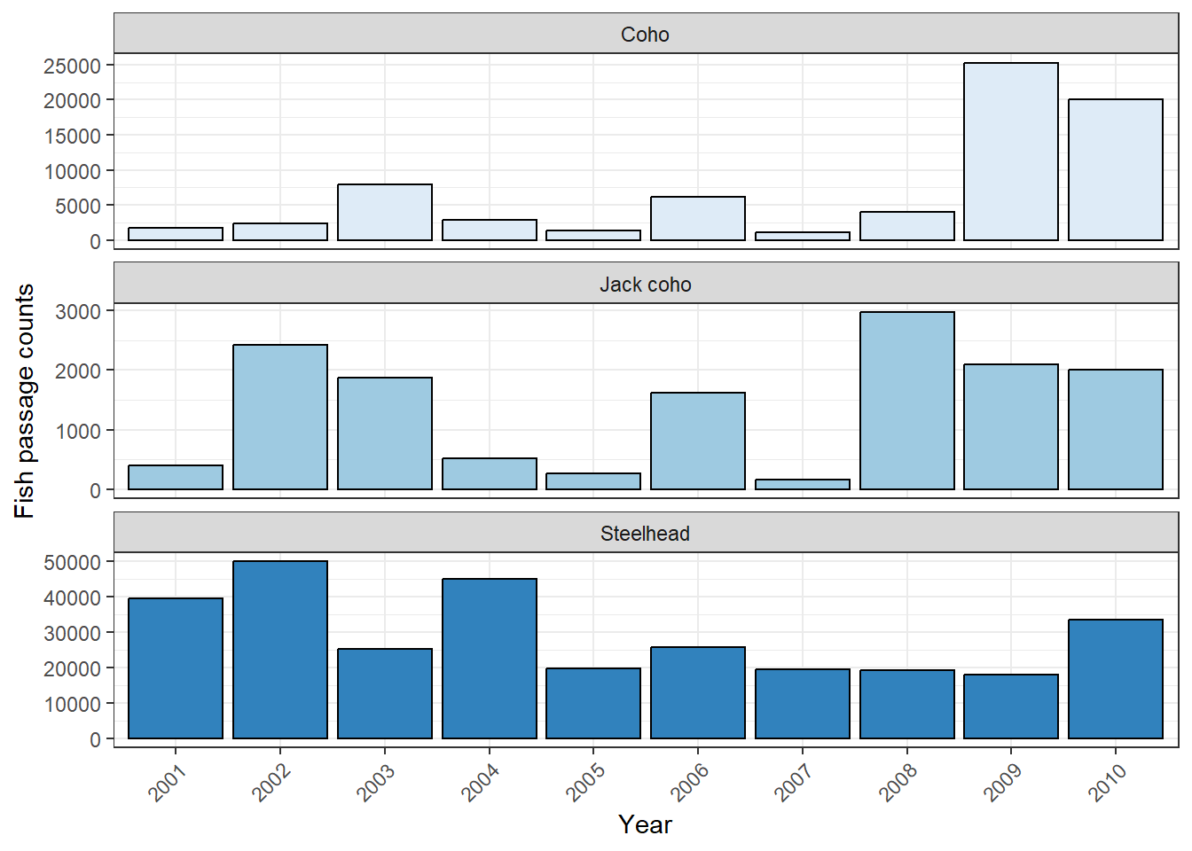

Figure 3: Annual totals for fish passage for coho (gray), jack coho (light blue), and steelhead (dark blue) salmon. Note the different y-axis values for each species to recognize the larger number of counts for steelhead and coho compared to jack coho.

Major Trends:

• I don’t see any clear trends in the annual totals by species from 2001-2010. Fish passage counts for coho salmon appear to be increasing overall throughout the decade, with a significant increase in 2009 and 2010. Jack coho counts follow a similar patter to the coho with recent increases, but with far less total fish passage counts overall.
• Steelhead salmon have the most overall and consistent counts year to year. There seems to be a slight decrease in their annual fish passage counts starting in 2005, but rebounded in 2010.

Acknowledgements

This assignment was created and organized by Casey O’Hara at the Bren School for ESM 244 (Advanced Data Analysis for Environmental Science & Management). ESM 244 is offered in the Master of Environmental Science & Management (MESM) program.